Why Pandas Matters
Pandas is one of the core tools for working with tabular data in Python.
For AI engineers, pandas is rarely the final destination.
It is the layer where raw information becomes usable system input.
That means pandas work is usually about:
loading data reliably
inspecting shape and quality
selecting useful subsets
deriving features
aggregating behavior
joining information from multiple sources
handling timestamps and text before downstream modeling
The official pandas getting-started guide organizes the learning path around those exact tasks, and this chapter follows that same progression in a book-friendly form.
Source: pandas getting started
Mental Model
In pandas, the main abstraction is the DataFrame.
You can think of it as:
a table with named columns
an index that identifies rows
vectorized operations over whole columns
a bridge between raw files and analytical or modeling code
The key shift is to stop thinking row by row.
Most good pandas code works column-wise and table-wise.
1. Creating And Inspecting Tables
Start with small, explicit tables so you can see the abstraction clearly.
import pandas as pd= pd.DataFrame("customer_id" : [101 , 102 , 103 , 104 ],"plan" : ["free" , "pro" , "team" , "pro" ],"monthly_spend" : [0 , 29 , 99 , 29 ],"active" : [True , True , False , True ],
0
101
free
0
True
1
102
pro
29
True
2
103
team
99
False
3
104
pro
29
True
Useful first questions:
What are the column names?
How many rows and columns are present?
What data types did pandas infer?
Are there missing values?
customer_id      int64
plan               str
monthly_spend    int64
active            bool
dtype: object
<class 'pandas.DataFrame'>
RangeIndex: 4 entries, 0 to 3
Data columns (total 4 columns):
 #   Column         Non-Null Count  Dtype
---  ------         --------------  -----
 0   customer_id    4 non-null      int64
 1   plan           4 non-null      str
 2   monthly_spend  4 non-null      int64
 3   active         4 non-null      bool
dtypes: bool(1), int64(2), str(1)
memory usage: 232.0 bytes
2. Reading And Writing Data
The pandas docs emphasize read_* functions and to_* methods as the main I/O interface.
That is a strong pattern to internalize:
input usually starts with pd.read_*
output usually ends with .to_*()
Common examples include:
pd.read_csv(...)pd.read_json(...)pd.read_parquet(...)df.to_csv(...)
For this repo, the most common beginner workflow will likely be CSV-based.
from io import StringIO= pd.DataFrame("event_id" : [1 , 2 , 3 ],"event_type" : ["click" , "purchase" , "click" ],"value" : [0.0 , 120.0 , 0.0 ],buffer = StringIO()buffer , index= False )buffer .seek(0 )= pd.read_csv(buffer )
0
1
click
0.0
1
2
purchase
120.0
2
3
click
0.0
3. Selecting Subsets
Selection is one of the first places where pandas becomes expressive.
0    free
1     pro
2    team
3     pro
Name: plan, dtype: str
"customer_id" , "monthly_spend" ]]
0
101
0
1
102
29
2
103
99
3
104
29
"monthly_spend" ] > 0 , ["customer_id" , "plan" , "monthly_spend" ]]
1
102
pro
29
2
103
team
99
3
104
pro
29
Use these patterns often:
df["col"] for one columndf[["a", "b"]] for multiple columnsdf.loc[row_filter, columns] for label-based selectiondf.iloc[...] for position-based selection
4. Creating Derived Columns
The official tutorial highlights derived columns because they are central to feature engineering.
"annualized_spend" ] = customers["monthly_spend" ] * 12 "is_paid" ] = customers["monthly_spend" ] > 0
0
101
free
0
True
0
False
1
102
pro
29
True
348
True
2
103
team
99
False
1188
True
3
104
pro
29
True
348
True
This matters for AI work because features are often transformations, not raw inputs.
5. Summary Statistics And Grouped Analysis
Before training or evaluating anything, summarize the data.
"monthly_spend" ].describe()
count     4.000000
mean     39.250000
std      42.113933
min       0.000000
25%      21.750000
50%      29.000000
75%      46.500000
max      99.000000
Name: monthly_spend, dtype: float64
"plan" )["monthly_spend" ].agg(["count" , "mean" , "max" ])
plan
free
1
0.0
0
pro
2
29.0
29
team
1
99.0
99
groupby is one of the most important pandas tools because it turns raw tables into behavioral summaries.
6. Reshaping Tables
Real systems often receive data in awkward formats.
Pandas gives you tools to reshape tables for analysis or modeling.
= pd.DataFrame("model" : ["baseline" , "baseline" , "tuned" , "tuned" ],"metric" : ["accuracy" , "f1" , "accuracy" , "f1" ],"score" : [0.81 , 0.77 , 0.86 , 0.83 ],
0
baseline
accuracy
0.81
1
baseline
f1
0.77
2
tuned
accuracy
0.86
3
tuned
f1
0.83
= "model" , columns= "metric" , values= "score" )
model
baseline
0.81
0.77
tuned
0.86
0.83
7. Combining Tables
Data rarely lives in one clean table.
You often need to join metadata, transactions, labels, or model outputs.
= pd.DataFrame("customer_id" : [101 , 102 , 103 , 104 ],"region" : ["US" , "IN" , "US" , "DE" ],= pd.DataFrame("customer_id" : [101 , 102 , 104 ],"monthly_spend" : [0 , 29 , 29 ],= "customer_id" , how= "left" )
0
101
US
0.0
1
102
IN
29.0
2
103
US
NaN
3
104
DE
29.0
The default mental model:
use merge for database-style joins
use concat to stack tables by rows or columns
8. Time Series Basics
Time is everywhere in AI systems:
logs
events
monitoring
feature histories
forecasting inputs
= pd.DataFrame("timestamp" : pd.to_datetime("2026-01-01 09:00:00" ,"2026-01-01 10:00:00" ,"2026-01-01 11:00:00" ,"requests" : [120 , 135 , 150 ],"hour" ] = traffic["timestamp" ].dt.hour
0
2026-01-01 09:00:00
120
9
1
2026-01-01 10:00:00
135
10
2
2026-01-01 11:00:00
150
11
Once a column is datetime-aware, pandas gives you rich .dt accessors for extracting useful temporal features.
9. Text Handling Basics
Text cleaning is another common preprocessing step.
= pd.DataFrame("review" : ["Great product!" ,"delivery delayed" ,"Works well for small teams" ,"review_lower" ] = reviews["review" ].str .lower()"contains_delivery" ] = reviews["review_lower" ].str .contains("delivery" )
0
Great product!
great product!
False
1
delivery delayed
delivery delayed
True
2
Works well for small teams
works well for small teams
False
The .str accessor makes string operations feel vectorized, just like numeric column operations.
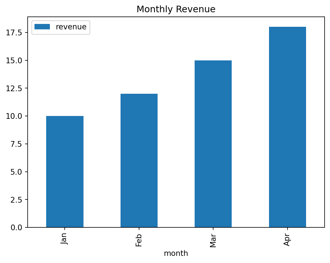
10. Plotting For Fast Inspection
The pandas getting-started guide includes plotting early because plots are useful for quick feedback loops.
= pd.DataFrame("month" : ["Jan" , "Feb" , "Mar" , "Apr" ],"revenue" : [10 , 12 , 15 , 18 ],= "month" , y= "revenue" , kind= "bar" , title= "Monthly Revenue" );
For serious visualization work, teams often move to Matplotlib, Seaborn, or Plotly.
But pandas plotting is perfect for fast inspection.
Common Beginner Mistakes
Writing row-by-row loops when vectorized column operations would be simpler
Forgetting to inspect dtypes before debugging results
Using chained indexing instead of clear loc selection
Merging tables without first checking key uniqueness
Treating missing values as a cosmetic issue instead of a data contract issue
Suggested Learning Path
If you want to learn pandas deeply, practice in this order:
Create and inspect DataFrame objects
Load and save CSV data
Filter rows and choose columns with loc
Add derived columns
Use groupby and aggregations
Reshape with pivot and melt
Join tables with merge
Work with datetime and string columns
Practice
The following notebooks are included in this repo as hands-on exercises:
Final Takeaway
Pandas is not just a library for tables.
It is a thinking tool for turning messy inputs into reliable structure.
That makes it foundational for data pipelines, feature work, evaluation slices, and AI system debugging.